Asteroids Simulator

This article explains how to develop a simulator of part of an Asteroids game in Geogebra using parametric curves based on position vectors. Note that this simulator is intended for exploring mathematical models and as such many of the details of a full Asteroids game have been abstracted.

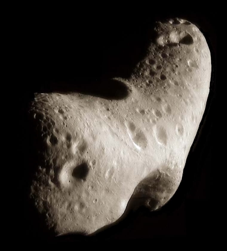
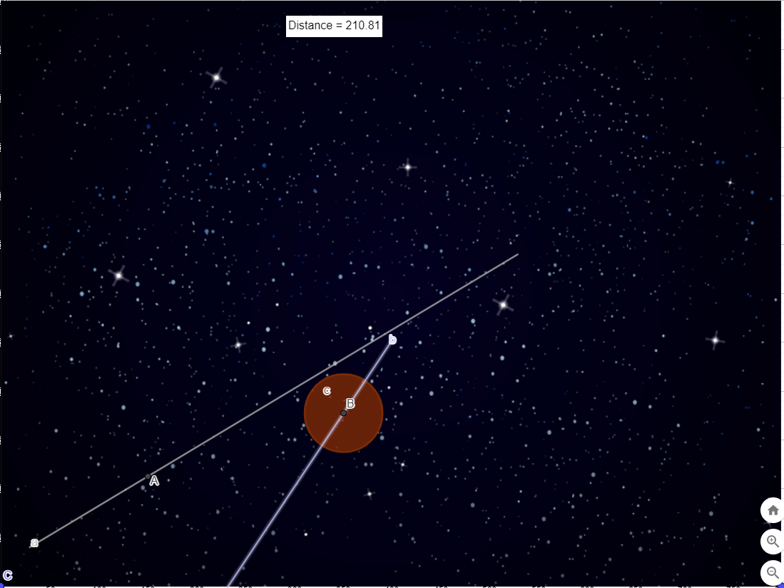
The animated gif image below is an example of a simple simulator developed in Geogebra. The large circle represents an Asteroid, while the smaller circle (dot) represents a missile that has been fired. The simulator demonstrates whether or not the missile hits the Asteroid and can be used to determine the minimum distance between the centre of the Asteroid and the missile.


Before we create the simulator, we provide a brief description of the main components of the Geogebra tool.
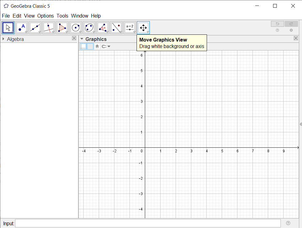
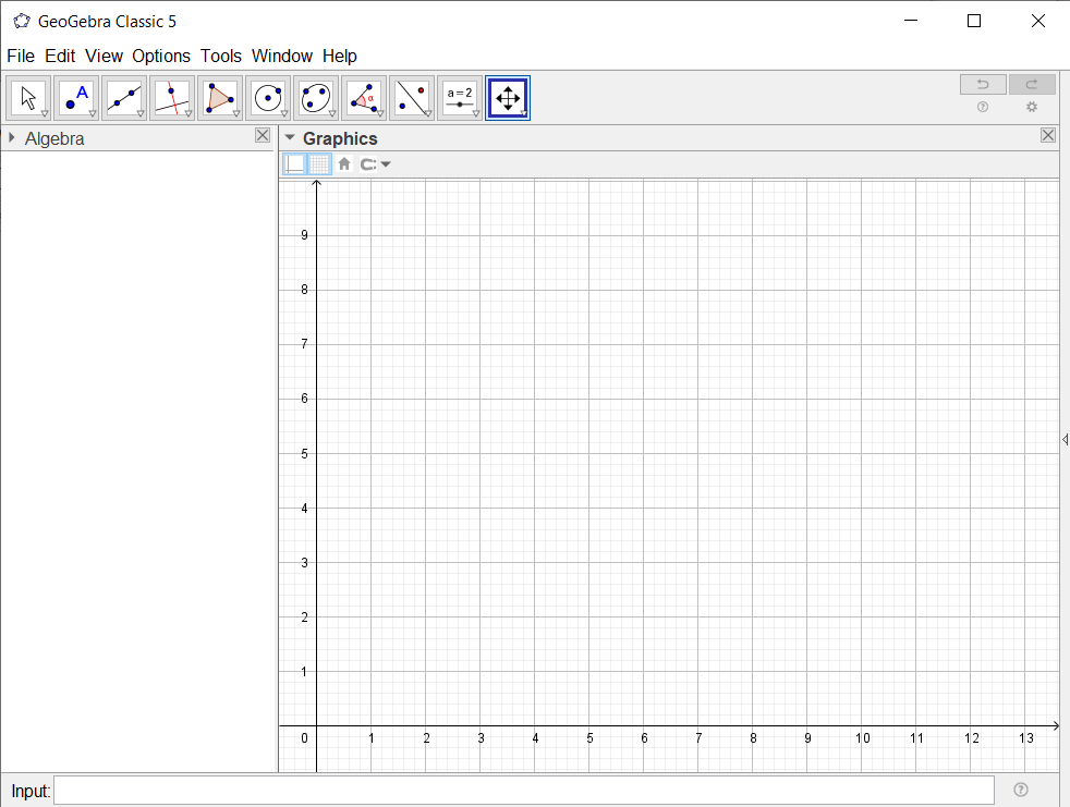
The screenshot below shows Geogebra Classic 6. On the left-hand side is the Algebra window. This is where we will input components of the mathematical model, including curves and points. The middle and main part of the display is the Graphic window, this is where the asteroids model will be displayed. The toolbar at the top of the screen provide access to the main geometric tools – in this article we some of these tools to create a slider, create a circle to represent an asteroid and add text showing the distance between two points.


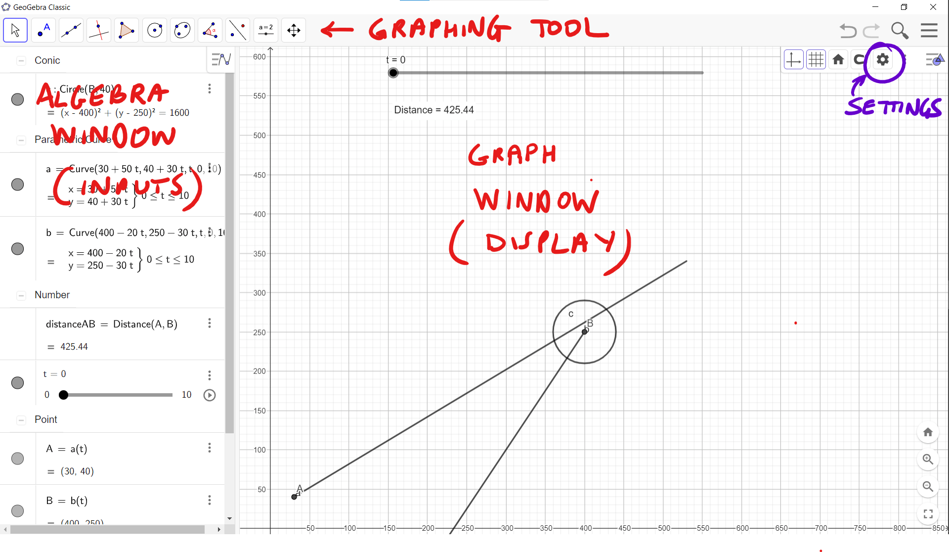
The highlighted settings button allows for the configuration of elements on the Graph window. Clicking on the background allows us to configure the background window.

Step 1: Screen dimensions

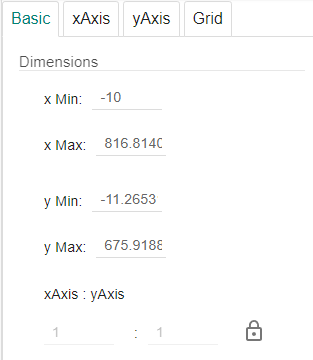
We begin by setting the screen dimensions. We assume that the game is played on a 4:3 aspect ratio with a resolution of 800 pixels wide and 600 pixels high. In Geogebra we will let 1 unit represent 1 pixel in the game. As such the range of x values will be between 0 and 800, while the range of y values will be between 0 and 600. Settings for this in Geogebra are shown below. Note that maximum x and y values go slightly beyond the range. Note also that we have a 1:1 ratio between the x and y scales. To access the configuration options for the background, click on the settings button.

Step 2: Representing time

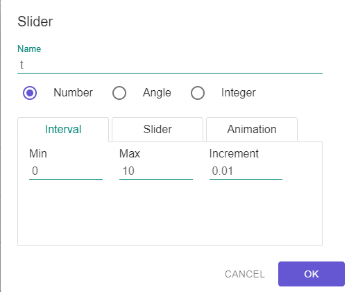
Time (in seconds) will be represented using a slider. For our example time will range from 0 to 10 seconds, with increments of 0.01 seconds. This slider is created using the slider tool.

The configuration options are shown in the following image.


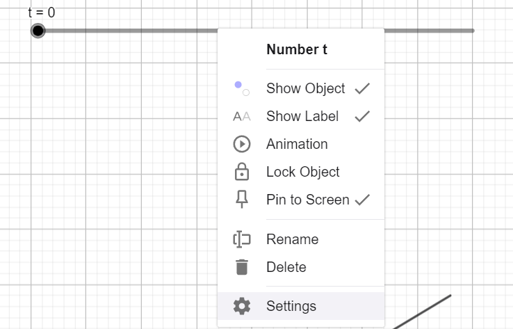
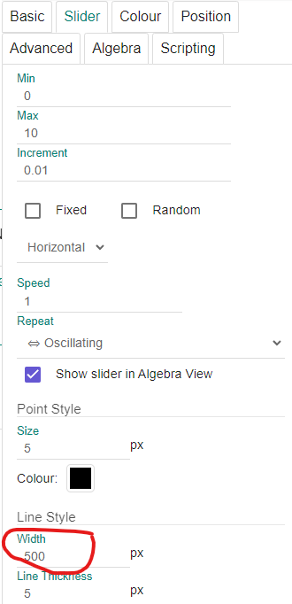
The width of the slider is increased from the default of 200 pixels to 500 pixels. To configure this right-click on the slider and select “Settings”.

The settings window for the slider is shown below with the updated width value highlighted.

Step 3: Modelling a missile

The missile in our example has an initial position of (30, 40) and a velocity vector of [50, 30]. The position vector (relative to the origin) is given as follows.
\vec{r_A} = [30, 40]+t[50,30]
To represent this position vector in Geogebra we use the Curve function. The function takes parameterised expressions for the x-coordinates and y-coordinates of points on the curve, together with parameter used in the expressions, and the lower and upper limits of values passed to the parameter. In this case we use the variable t as the parameter and set the range of values from 0 to 10. The input for this in Geogebra is as follows:

Curve(30+50t, 40+30t, t, 0, 10)

To trace the path of the missile at a particular time we create a new point representing the point on the curve for the current value of the time variable. The input for this in Geogebra is given below:

a(t)

The details of the curve and parameterised point should appear in Geogebra as shown in the screenshot below.

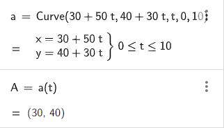
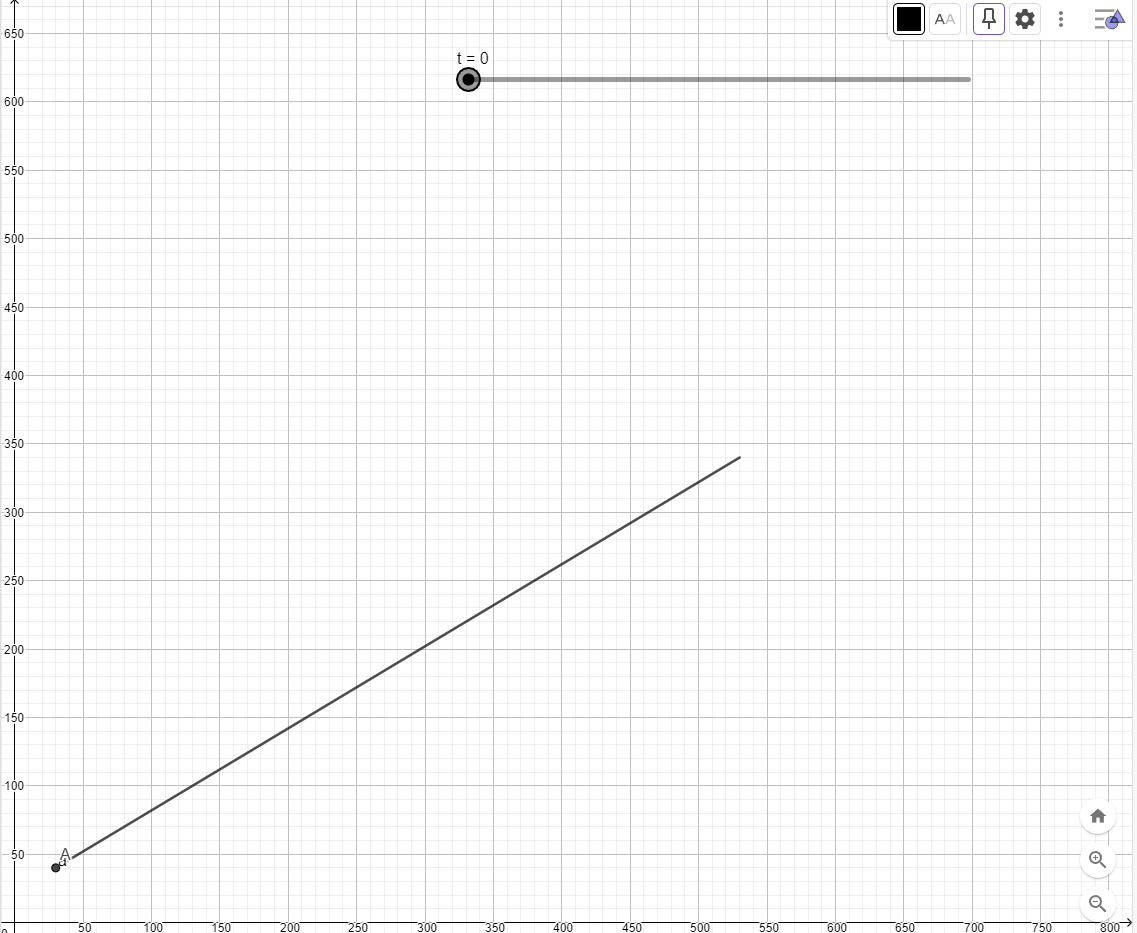
The graphing window should look like the screenshot below after the commands shown above have been entered. It shows the path that the missile will take over the 10 second time interval, together with the current position of the missile (shown as point A). The time variable has a value of 0 and the missile is at its starting position of (30, 40).

Step 4: Modelling an asteroid

Next we model an asteroid with an initial position of (400, 250) and a velocity vector of [-20, -30]. The asteroid will be modelled as a circle with a diameter of 80 pixels. The position vector (relative to the origin) of the asteroid is given as follows.
\vec{r_A} = [400, 250]+t[-20,-30]
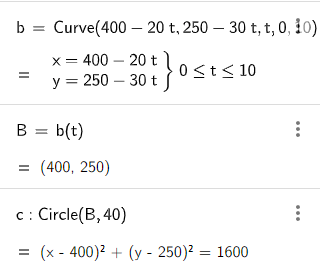
The path of the asteroid is modelled using the Curve function in Geogebra.

Curve(400-20t, 250-30t, t, 0, 10)

Next, the centre of the asteroid is modelled as a parameterised point.

b(t)

Finally, a circle whose centre is the parameterised point is created using the “Circle: Center and Radius” tool.

The radius of the circle is 40 pixels. The details of the curve, parameterised point and circle are shown in the screenshot below.

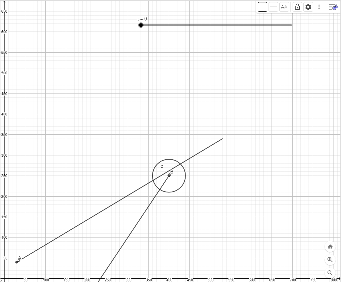
After these commands have been added the graphing window should look like the screenshot below.

Step 5: Tracking the distance between objects

To determine whether the missile hits the asteroid we will track the distance between the centres of these objects. We begin by choosing the “Distance or Length” tool and selecting the point representing the missile and the point representing the centre of the asteroid (points A and B). This will create a distance calculation object together with a text object to display the distance.

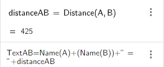
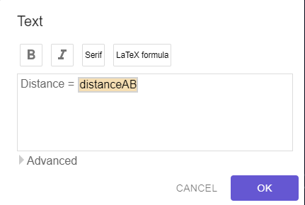
Double-clicking on the text element pops up a window allowing us to edit the text. In this case we change the text on the left-hand side of the equal sign as shown in the screenshot below.

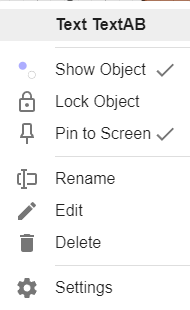
We then open the settings for the text object and click on the Pin to Screen option. Selecting this lets us move the text to the top of the screen.

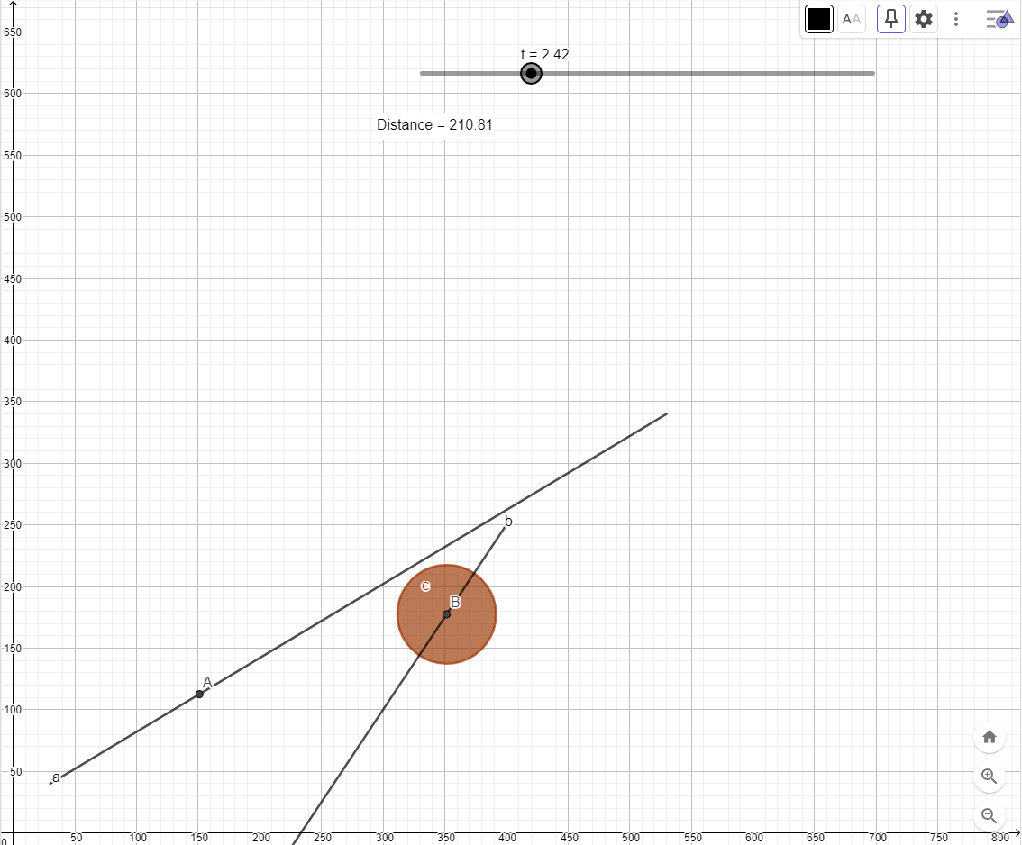
After these steps have been completed the Graphic Window will look like the screenshot below (note this also includes a change in colour for the asteroid which is accessed by clicking on the asteroid object and then selecting settings).

Extra bling

The look of the simulator can be improved by adding a space background. This is done by choosing the “Image” tool.

In this case an image that has the correct 4:3 aspect ratio is chosen. The image appears in the middle of the Graph window as shown in the following screenshot.

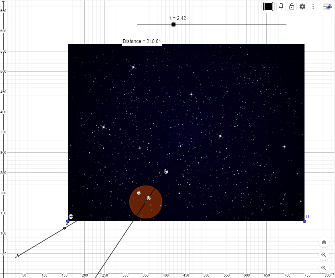
The anchor points of the image (points C and D) are so that the image covers an 800×600 area.

The final result is shown in the following screenshot.

Investigating Trigonometric Ratios

This classroom activity uses the Geogebra tool to derive and explore the trigonometric ratios. A right-angled triangle with given angles is created precisely and enlargements of this triangle are created. Ratios between sides are calculated and compared across all the triangles. These ratios are then compared with the sine, cosine and tangent trigonometric ratios for the given angles.

In this investigation you will explore similar right-angled triangles. Each student will explore a triangle with different angles.

  1. Record the angle assigned by your teacher, or randomly select an
    angle between 30 and 75.
  2. Open a new Geogebra window, ensuring that the grid and axes are
    both showing.

Create a right-angled triangle, with one of the angles matching your
assigned angle, using the following steps:

  1. Create a line using the “Line” tool and a second perpendicular
    line using the “Perpendicular Line” tool. The intersection of these two
    lines will form the right-angle of our right-angled triangle.

  2. Create an angle with the size specified in (1) using the “Angle
    with Given Size” tool

    1. Create a point D on the first line using the “Point on Object”
      tool. The point should appear to the right of the intersection between
      the two lines as shown in the diagram below.
    2. Select the “Angle with Given Size” tool
    3. Click on point A
    4. Click on point D
    5. Select clockwise for the angle measure
    6. Enter the size of the angle (as given in (1))
    7. Use the “Line” tool to connect the two newly created points
      (points A’ and D in the diagram below).

  3. Create two additional points (E and F below) at the intersections
    of the lines using the “Intersect” tool.
  4. Form a triangle using the “Polygon” tool that connects the three
    intersection points.

  5. Use the “Angle” tool to show the three angles within the
    triangle.
  6. Hide the unnecessary lines and points used in creating the
    triangle by de-selecting the objects in the Algebra View.

  7. Measure the lengths of each side in the triangle.
  8. Save your file at this stage (if not done so already) and export
    an PNG image file of your right-angled triangle.
  9. Using the enlargement transformation method used in Part 1,
    create enlargements of your right-angled triangle with scale factors of
    2 and 4.
  10. Measure all sides and angles in the two enlargements. Save your
    file and export a PNG image file.
  11. Record all angles, side lengths and side ratios in a table like
    the following. You should record the lengths to 5 decimal places. Go to
    Rounding under the Options menu and change the rounding settings.

    Angle Opp Adj Hyp \dfrac{Opp}{Adj} \dfrac{Opp}{Hyp} \dfrac{Adj}{Hyp}
    Triangle 1
    Triangle 2
    Triangle 3

The angle is the one given in (1). Opposite, adjacent and hypotenuse
are all measured from the given angle as shown in the following
diagram.

  1. Comment on the ratios between the three sides for the three
    triangles as shown in the table created in step (13).
  2. For your given angle, use your calculator to complete the
    following table.

    tan  θ sin  θ cos  θ
    θ=  
  3. Using the tables from (13) and (15) complete the following rules

    \tan \theta =

    \sin \theta =

    \cos \theta =

  4. Repeat step (13) using the other acute angle in your triangle,
    recording your measurements and calculations in a new table.
  5. Using the tables from (13), (15) and (17) define a rule(s) that
    connects the sine and cosine functions.

Investigating similar triangles using Geogebra

To explore properties of similar triangles we will apply enlargement transformations to a triangle using the Geogebra tool.


You can either use the online version of Geogebra or you can download Geogebra Classic 5 or Geogebra Classic 6. Note that the screen shots shown below are based on Geogebra Classic 5, however Geogebra Classic 6 is very similar.

  1. Open a new Geogebra window, ensuring that the grid and axes are shown.

  2. Using the “Move Graphics View” tool, move the window so that the window is focussed on the 1st quadrant of the Cartesian plane.

  3. Use the “Point” tool to create a point at the origin of the Cartesian plane (0,0). This is referred to as the enlargement origin.

  4. Use the “Polygon” tool to create a triangle with all three vertices in the 1st quadrant.

  5. Use the “Line” tool to create three lines that each pass through the transformation origin and one of the vertices of the triangle.

  6. Use the “Enlarge from Point” tool to create a second triangle which is an enlargement of the first.
    1. Select the “Enlarge from Point” tool

    2. Click on the original triangle
    3. Select the enlargement origin
    4. Enter a scale factor of 2

  7. Measure the three internal angles of the first triangle

    1. Select the “Angle” tool

    2. Click within the first triangle – all three angles should be
      marked.

  8. Repeat the above steps to measure all three internal angles of
    the second triangle.

  9. Record your measurements in a table like the one below:

    Angle 1 Angle 2 Angle 3
    Triangle 1
    Triangle 2
  10. Measure the three sides of the first triangle

    1. Select the “Distance or Length” tool

    2. Select the two vertices at either end of the side

    3. Repeat for the other two sides

  11. Repeat the above steps for the second triangle.

  12. Record your measurements in a table like the one below. Include
    calculations of the ratios between side lengths for each of the two
    triangles.

    Side 1 Side 2 Side 3 Side 1 ÷
    Side 2
    Side 1 ÷
    Side 3
    Side 2 ÷
    Side 3
    Triangle 1
    Triangle 2
  13. Calculate the area of the first triangle using the “Area” tool

    1. Select the “Area” tool

    2. Click on the triangle

  14. Repeat for the second triangle.

  15. Insert your measurements of area in a table like the one
    below:

    Area
    Triangle 1
    Triangle 2
  16. Save your Geogebra file as “enlargement_transformation.ggb” using
    “Save” from the “File” menu.

  17. Export your enlargement diagram to a “PNG” file using
    “Export”->”Graphics View” from the “File” menu.

  18. With reference to your measurements in the three tables, comment
    on how the angles, side lengths, rations between sides, and area are
    affected by an enlargement transformation with a scale factor of
    2.

  19. Predict what will happen to the angles, side lengths, ratios
    between sides, and area, if the original triangle is enlarged by a scale
    factor of 3.

  20. Use Geogebra to test your prediction, include an exported image
    file as evidence.

  21. Summarise your findings with four hypotheses relating to the
    angles, side lengths, ratios between sides, and area of enlarged
    triangles with a scale factor of n.