Introduction
In this series of tutorials we explain how to develop a Measurement toolkit which provides functions for converting units of measurement and calculating the surface area and volume of a range of 3d shapes.
A screenshot showing the Measurement toolkit is given below showing the unit conversion capabilities of the tool.
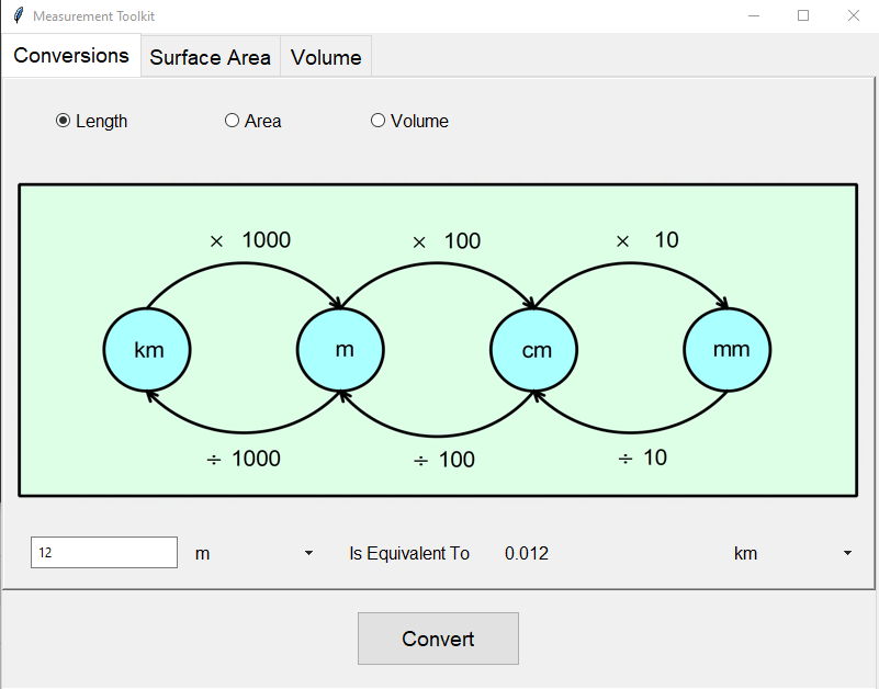
Unit conversions in the Measurement Toolkit
Initial setup
The starting point for the development of the Measurement Toolkit is to download the initial source code files for the Measurement Toolkit. This zip file should be downloaded and extracted to a suitable location. These files provide the basic skeletal code for the application. It includes graphical user interface (GUI) code, together with stubs for the functions that do the conversions and calculations.
The files are listed below, with full code listings that can be expanded and view. We will describe each of these files in more detail in later parts of this tutorial as required.
convert_units.py – will contain functions for carrying out unit conversions. Code is provided in this file for converting units of length, however several errors have been included which need to be found through testing and fixed. Stubs (incomplete functions) for converting area and volume units are also given.
def convert_length_unit(value,inunit, outunit):
if (inunit==outunit):
result=value
elif (inunit=="m") & (outunit=="mm"):
result=value*1000
elif (inunit=="m") & (outunit=="cm"):
result=value*10
elif (inunit=="m") & (outunit=="km"):
result=value*1000
elif (inunit=="km") & (outunit=="mm"):
result=value*1000000
elif (inunit=="km") & (outunit=="cm"):
result=value*10000
elif (inunit=="km") & (outunit=="m"):
result=value*1000
elif (inunit=="cm") & (outunit=="mm"):
result=value*100
elif (inunit=="cm") & (outunit=="m"):
result=value/100
elif (inunit=="cm") & (outunit=="km"):
result=value/100*1000
elif (inunit=="mm") & (outunit=="cm"):
result=value/10
elif (inunit=="mm") & (outunit=="m"):
result=value/1000
elif (inunit=="mm") & (outunit=="km"):
result=value/1000*1000
return result
def convert_area_unit(value,inunit,outunit):
return 0
def convert_volume_unit(value,inunit,outunit):
return 0
convert_units_tester.py – will contain test cases to check the correctness of the unit conversion functions. Test cases have been written for converting from metres to other units. Using the same syntax you will be required to complete the other test cases.
import unittest
from convert_units import *
class TestConvertUnits(unittest.TestCase):
def test_m_to_mm(self):
self.assertEqual(convert_length_unit(0.23,"m","mm"),230)
def test_m_to_cm(self):
self.assertEqual(convert_length_unit(0.25,"m","cm"),25)
def test_m_to_m(self):
self.assertEqual(convert_length_unit(178,"m","m"),178)
def test_m_to_km(self):
self.assertEqual(convert_length_unit(19000,"m","km"),19)
if __name__ == '__main__':
unittest.main()
mathtoolkit.py – the main program file, containing of the GUI code and user configurable code allowing additional shapes to be added to the surface area and volume calculator parts of the tool
from tkinter import *
from tkinter import ttk
from convert_units import *
from surface_area import *
from volume import *
from PIL import Image,ImageTk
import math
def convert_units_and_display():
if (unitsvar.get()==1):
converted=convert_length_unit(float(unitval.get()),funitvar.get(),tunitvar.get())
elif (unitsvar.get()==2):
converted=convert_area_unit(float(unitval.get()),funitvar.get(),tunitvar.get())
elif (unitsvar.get()==3):
converted=convert_volume_unit(float(unitval.get()),funitvar.get(),tunitvar.get())
convertedval.set(str(converted))
def change_unit_options():
m1=foptnmenu['menu']
m1.delete(0,END)
m2=toptnmenu['menu']
m2.delete(0,END)
if (unitsvar.get()==2):
newvalues=['mm2','cm2','m2','km2']
funitvar.set("m2")
tunitvar.set("m2")
image=Image.open("Images/area_convert.png").resize((780,300))
img=ImageTk.PhotoImage(image)
cimage_label.configure(image=img)
cimage_label.image=img
elif(unitsvar.get()==3):
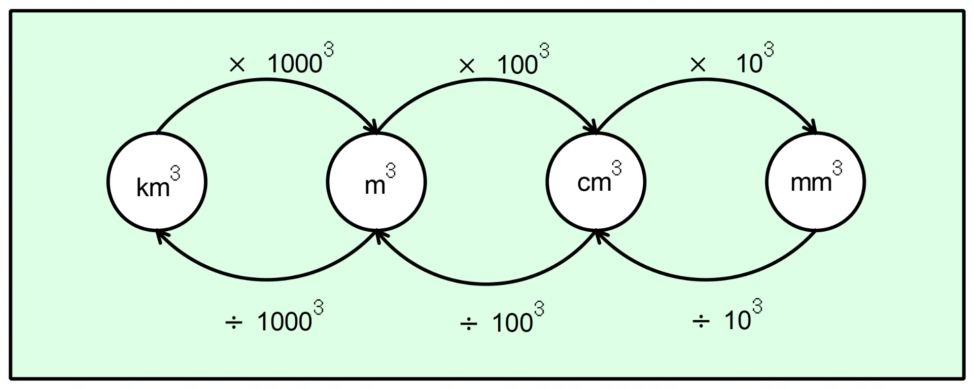
newvalues=['mm3','cm3','m3','km3']
funitvar.set("m3")
tunitvar.set("m3")
image=Image.open("Images/volume_convert.png").resize((780,300))
img=ImageTk.PhotoImage(image)
cimage_label.configure(image=img)
cimage_label.image=img
else:
newvalues=['mm','cm','m','km']
funitvar.set("m")
tunitvar.set("m")
image=Image.open("Images/length_convert.png").resize((780,300))
img=ImageTk.PhotoImage(image)
cimage_label.configure(image=img)
cimage_label.image=img
for val in newvalues:
m1.add_command(label=val,command=lambda v=funitvar,l=val:funitvar.set(l))
m2.add_command(label=val,command=lambda v=tunitvar,l=val:tunitvar.set(l))
def display_shape_sa(self):
sproperties=sa_shapes[shapevar.get()]
refresh_surface_area(sproperties[0],
sproperties[1])
def calc_surface_area():
arglist=""
for i in range(0,len(valarray)-1):
arglist=arglist+"{0},".format(valarray[i].get())
arglist=arglist+"{0}".format(valarray[len(valarray)-1].get())
answer=(eval(sa_shapes[shapevar.get()][2]+"("+arglist+")"))
sa_text.set("Surface Area of {0} is {1:.2f} units^2".format(shapevar.get(),answer))
def refresh_surface_area(varlist,imageloc):
valarray.clear()
for l in range(0,len(varlabels)):
varlabels[l].destroy()
for l in range(0,len(varentries)):
varentries[l].destroy()
for i in range(0,len(varlist)):
valarray.append(StringVar(main))
lab=ttk.Label(vframe,text="{0}=".format(varlist[i]))
lab.grid(row=i+1,column=0,pady=20,sticky=W)
varlabels.append(lab)
entry=ttk.Entry(vframe,width=20,textvariable=valarray[i])
entry.grid(row=i+1,column=1,sticky=W)
varentries.append(entry)
image=Image.open(imageloc).resize((400,400))
img=ImageTk.PhotoImage(image)
image_label.configure(image=img)
image_label.image=img
def display_shape_vol(self):
vproperties=vol_shapes[vshapevar.get()]
refresh_volume(vproperties[0],
vproperties[1])
def calc_volume():
arglist=""
for i in range(0,len(vvalarray)-1):
arglist=arglist+"{0},".format(vvalarray[i].get())
arglist=arglist+"{0}".format(vvalarray[len(vvalarray)-1].get())
answer=(eval(vol_shapes[vshapevar.get()][2]+"("+arglist+")"))
vol_text.set("Volume of {0} is {1:.2f} units^3".format(vshapevar.get(),answer))
def refresh_volume(varlist,imageloc):
vvalarray.clear()
for l in range(0,len(vvarlabels)):
vvarlabels[l].destroy()
for l in range(0,len(vvarentries)):
vvarentries[l].destroy()
for i in range(0,len(varlist)):
vvalarray.append(StringVar(main))
lab=ttk.Label(vframe2,text="{0}=".format(varlist[i]))
lab.grid(row=i+1,column=1,pady=20)
vvarlabels.append(lab)
entry=ttk.Entry(vframe2,width=20,textvariable=vvalarray[i])
entry.grid(row=i+1,column=2)
vvarentries.append(entry)
image=Image.open(imageloc).resize((400,400))
img=ImageTk.PhotoImage(image)
vimage_label.configure(image=img)
vimage_label.image=img
####################
## Top level GUI setup
######################
main=Tk()
main.title('Measurement Toolkit')
main.geometry('800x600')
rows=0
main.grid_rowconfigure(0, weight=1)
main.grid_columnconfigure(0, weight=1)
style = ttk.Style(main)
style.configure('TRadiobutton', font=('Helvetica', 12))
style.configure('TNotebook.Tab', font=('Helvetica', 14), padding=5)
style.configure('TButton', font=('Helvetica', 14), padding=10)
style.configure('TLabel', font=('Helvetica', 12))
style.configure('TEntry', font=('Helvetica', 12), padding=5)
style.configure('TMenubutton', font=('Helvetica', 12), padding=5)
nb=ttk.Notebook(main)
nb.grid(row=0,sticky="nesw")
page1=ttk.Frame(nb)
nb.add(page1,text='Conversions')
page2=ttk.Frame(nb)
nb.add(page2,text='Surface Area')
page3=ttk.Frame(nb)
nb.add(page3,text='Volume')
##################
## Conversions
###################
page1.rowconfigure(0,weight=2)
page1.rowconfigure(1,weight=1)
page1.columnconfigure(0,weight=1,uniform=1)
unitsvar=IntVar()
unitsvar.set(1)
cframe=ttk.Frame(page1,relief=RAISED,padding=5)
cframe.grid(row=0,column=0,sticky="nesw")
cframe.columnconfigure((0,1,2,3,4),weight=1)
cframe.rowconfigure(1,weight=1)
cframe.rowconfigure((0,2),weight=1)
cimage_label=ttk.Label(cframe)
cimage_label.grid(row=1,column=0,columnspan=5,sticky="ew")
image=Image.open("Images/length_convert.png").resize((780,300))
img=ImageTk.PhotoImage(image)
cimage_label.configure(image=img)
cimage_label.image=img
ttk.Radiobutton(cframe,text="Length",variable=unitsvar,value=1,command=change_unit_options).grid(row=0,column=0,pady=10)
ttk.Radiobutton(cframe,text="Area",variable=unitsvar,value=2,command=change_unit_options).grid(row=0,column=1,pady=10)
ttk.Radiobutton(cframe,text="Volume",variable=unitsvar,value=3,command=change_unit_options).grid(row=0,column=2,pady=10)
funitvar=StringVar(main)
tunitvar=StringVar(main)
unitchoices=['mm','cm','m','km']
unitval=StringVar(main)
unitval.set("0")
convertedval=StringVar(main)
convertedval.set("0")
ttk.Label(cframe,text='Is Equivalent To').grid(row=2,column=2,padx=5,pady=5)
uentry=ttk.Entry(cframe,width=20,textvariable=unitval)
uentry.grid(row=2,column=0,sticky='E')
foptnmenu=ttk.OptionMenu(cframe,funitvar,'m',*unitchoices)
foptnmenu.configure(width=10)
foptnmenu.grid(row=2,column=1)
convertLabel=ttk.Label(cframe,textvariable=convertedval,width=20)
convertLabel.grid(row=2,column=3)
toptnmenu=ttk.OptionMenu(cframe,tunitvar,'m',*unitchoices)
toptnmenu.configure(width=10)
toptnmenu.grid(row=2,column=4)
convertButton=ttk.Button(page1,text="Convert",
command=convert_units_and_display)
convertButton.grid(row=1,column=0)
#################
## Surface Area
###################
sa_shapes={}
##
## ADD NEW SHAPES HERE FOR SURFACE AREA
##
sa_shapes['Cube']=[['l'],"Images/cube.png","calc_cube_sa"]
sa_shapes['Rectangular Prism']=[['l','w','h'],"Images/rect_prism.png","calc_rprism_sa"]
##
## DO NOT EDIT BELOW HERE
##
page2.rowconfigure(0,weight=1)
page2.rowconfigure(1,weight=1)
page2.rowconfigure(2,weight=1)
page2.rowconfigure(3,weight=1)
page2.columnconfigure(0,weight=1,uniform=1)
shapechoices=sa_shapes.keys()
shapevar=StringVar(main)
shapevar.set('Cube')
shapeoptnmenu=ttk.OptionMenu(page2,shapevar,"Cube",*shapechoices,command=display_shape_sa)
shapeoptnmenu.configure(width=30)
shapeoptnmenu.grid(row=0,column=0,sticky=W)
vframe=ttk.Frame(page2,relief=RAISED,padding=10)
vframe.grid(row=1,column=0,sticky=NSEW)
ttk.Label(vframe,text="Variables").grid(row=0,column=1,padx=20)
iframe=ttk.Frame(page2,relief=RAISED,padding=5)
iframe.grid(row=1,column=1,sticky=NSEW)
valarray=[]
varlabels=[]
varentries=[]
image_label=ttk.Label(iframe,background='white')
image_label.grid(row=0,column=0)
display_shape_sa(main)
sa_text=StringVar()
sa_text.set("Press Calculate button")
ttk.Label(page2,textvariable=sa_text).grid(row=2,column=0, columnspan=2, sticky=W)
ttk.Button(page2,text="Calculate",command=calc_surface_area).grid(row=3,column=0,columnspan=2)
################
## Volume
################
vol_shapes={}
##
## ADD NEW SHAPES HERE FOR VOLUME
##
vol_shapes['Cube']=[['l'],"Images/cube.png","calc_cube_vol"]
vol_shapes['Rectangular Prism']=[['l','w','h'],"Images/rect_prism.png","calc_rprism_vol"]
##
## DO NOT EDIT BELOW HERE
##
page3.rowconfigure(0,weight=1)
page3.rowconfigure(1,weight=1)
page3.rowconfigure(2,weight=1)
page3.rowconfigure(3,weight=1)
page3.columnconfigure(0,weight=1,uniform=1)
vshapechoices=vol_shapes.keys()
vshapevar=StringVar(main)
vshapevar.set('Cube')
vshapeoptnmenu=ttk.OptionMenu(page3,vshapevar,"Cube",*vshapechoices,command=display_shape_vol)
vshapeoptnmenu.configure(width=30)
vshapeoptnmenu.grid(row=0,column=0,sticky=W)
vframe2=ttk.Frame(page3,relief=RAISED)
vframe2.grid(row=1,column=0,sticky=NSEW)
ttk.Label(vframe2,text="Variables").grid(row=0,column=1,columnspan=2,padx=20)
iframe2=ttk.Frame(page3,relief=RAISED,padding=5)
iframe2.grid(row=1,column=1,sticky=NSEW)
vvalarray=[]
vvarlabels=[]
vvarentries=[]
vimage_label=ttk.Label(iframe2,background='white')
vimage_label.grid(row=0,column=0)
display_shape_vol(main)
vol_text=StringVar()
vol_text.set("Press Calculate button")
ttk.Label(page3,textvariable=vol_text).grid(row=2,column=0, columnspan=2, sticky=W)
ttk.Button(page3,text="Calculate",command=calc_volume).grid(row=3,column=0,columnspan=2)
main.mainloop()
surface_area.py – will contain the functions for calculating the surface area of various 3d shapes
import math
def calc_cube_sa(length):
return 6*(length)**2
def calc_rprism_sa(length,width,height):
return 0
surface_area_tester.py – will contain test cases to check the correctness of the surface area calculation functions
import unittest
from surface_area import *

class TestSurfaceArea(unittest.TestCase):
    def test_calc_cube_sa(self):
        self.assertEqual(calc_cube_sa(5),150)
        self.assertAlmostEqual(calc_cube_sa(3.275),64.35,2)

if __name__ == '__main__':
    unittest.main()
volume.py – will contain the functions for calculating the volume of various 3d shapes
import math

def calc_cube_vol(l):
    return l**3

def calc_rprism_vol(l,w,h):
    return 0
volume_tester.py – will contain test cases to check the correctness of the volume calculation functions
import unittest
from volume import *

class TestVolume(unittest.TestCase):
    def test_calc_cube_vol(self):
        self.assertEqual(calc_cube_vol(5),125)

if __name__ == '__main__':
    unittest.main()
Images – stores the image files that will be used to represent the 3d shapes, together with the unit conversion diagrams
To run the program you will also need to install the pillow package in Python using the following command:
pip install pillow pip --trusted-host pypi.org --trusted-host files.pythonhosted.org
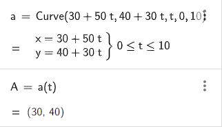
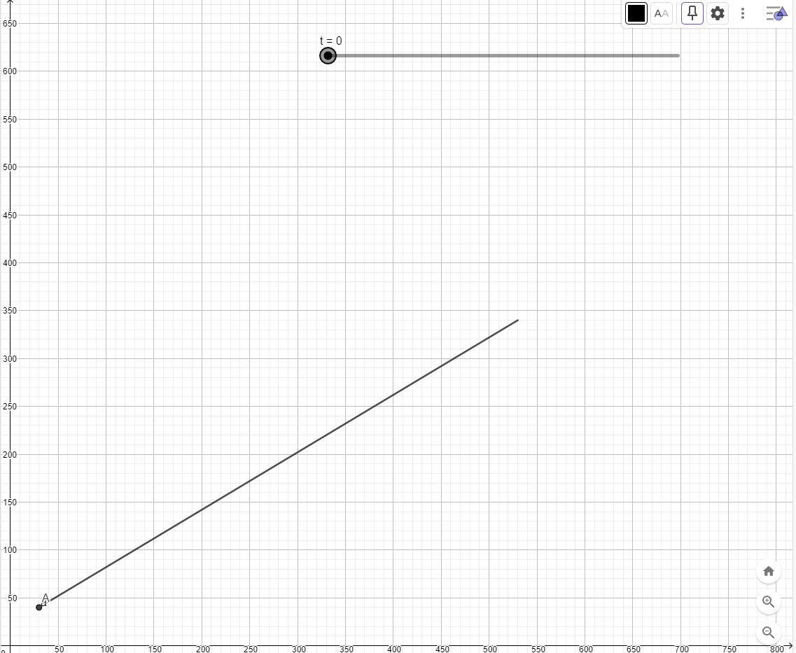
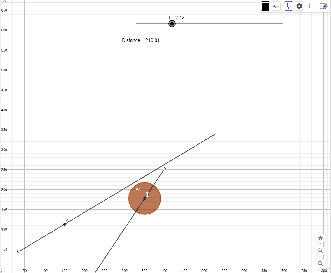
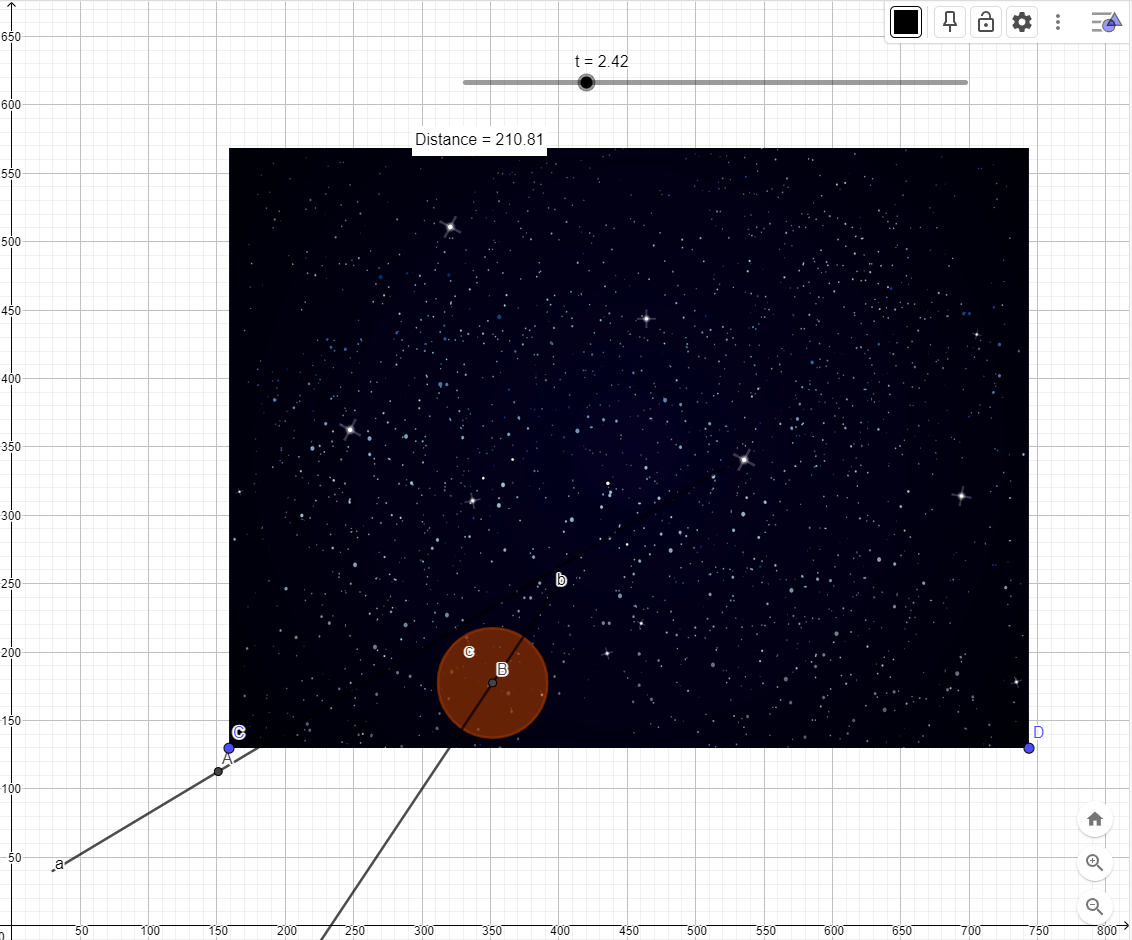
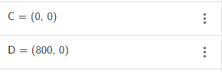
![\vec{r_A} = [30, 40]+t[50,30]](https://s0.wp.com/latex.php?latex=%5Cvec%7Br_A%7D+%3D+%5B30%2C+40%5D%2Bt%5B50%2C30%5D&bg=ffffff&fg=000000&s=0 "\vec{r_A} = [30, 40]+t[50,30]")
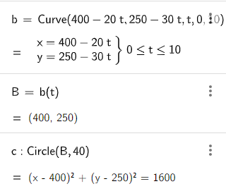
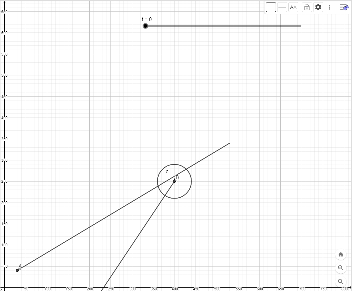
![\vec{r_A} = [400, 250]+t[-20,-30]](https://s0.wp.com/latex.php?latex=%5Cvec%7Br_A%7D+%3D+%5B400%2C+250%5D%2Bt%5B-20%2C-30%5D&bg=ffffff&fg=000000&s=0 "\vec{r_A} = [400, 250]+t[-20,-30]")


")

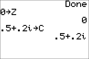
 = 0.5+0.2i")
^2+(0.5+0.2i) = 0.71+0.4i")

^2+(0.5+0.2i) = 0.8441+0.768i")

