In this tutorial we present the development of a GUI-based application in Python using tkinter. A variety of widgets are covered including: labels, entries, buttons, spinboxes, combo boxes, radio buttons, check buttons, scale and calendars. The focus for this tutorial is on constructing the view layer (how the application appears) with minimal development of the underlying logic.
Application Design
Before we write any code we need to design the layout for our application.
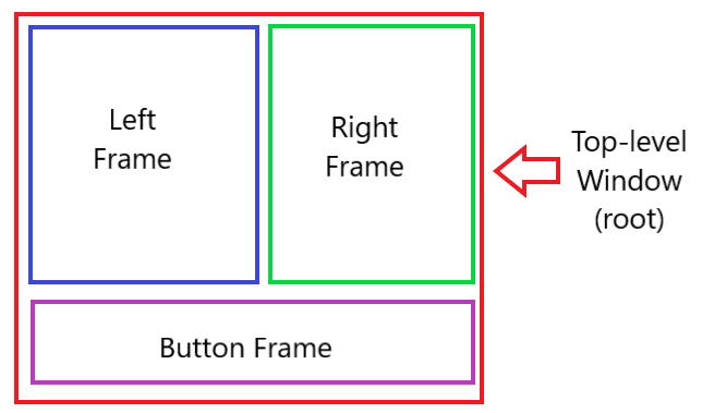
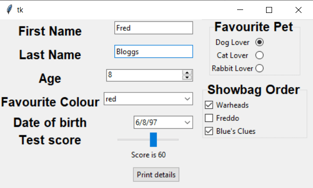
For this example we will divide our application into three main parts. The left frame will contain the entry (input) components of our application. The right frame will include additional configuration components in the form of radio buttons and checkbuttons.
The button frame will contain command buttons. An overview of the layout is shown below.
Step 1: The top-level window
We begin by creating the top-level window (root) for the application. Lines 1 and 2 of the code import the tkinter package, that contains all of the basic interface widgets, together with the ttk extension package, which includes enhanced and additional widgets.
The main control window of the application is created on line 5 of the code. The last line of the code (line 17) initialises the control loop for the GUI application – this line should always occur at the end of the code listing.
Lines 7-15 create frames for the three main parts of the application interface as explained above. To ensure that the button frame spans all of the application window we use the columnspan option.
from tkinter import *
from tkinter.ttk import *

# create the main application window
root = Tk()

# create a frame for a variety of entry and scale widgets
left_frame = Frame(root)
left_frame.grid(row=0, column=0)

right_frame = Frame(root)
right_frame.grid(row=0, column=1)

button_frame = Frame(root)
button_frame.grid(row=1, column=0, columnspan=2)

root.mainloop()
Step 2: Labels and Entries
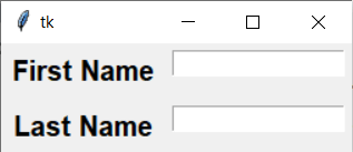
In the next step we add two pairs of labels and entry widgets that will allow the user to enter their first name and last name.
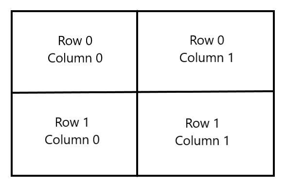
These widgets are packed using the grid packing system within the left frame as shown in the diagram below. The grid consists of two rows and two columns, with the numbering starting at 0 for both the row and column.
Labels are added to the application using the Label widget as seen in line 2 below. The font command is used to change the appearance of the text, using a size larger than the default and representing the text using boldface. The Entry widget is used to get input from the user, in this case to get their first and last names. Both of the Entry widgets are associated with a text variable. When text is entered in the entry box the value of the text variable is updated automatically. Both of the text variables are mapped string variables.
The following code is added to the previous code after the creation of the left, right and button frames and before the final line of code.
# label and entry widgets used to enter information. Values linked to string variable.
first_name_label = Label(left_frame, text="First Name", font=("-size", 15, "-weight", "bold"))
first_name_label.grid(row=0, column=0, padx=5, pady=5)
first_name = StringVar()
first_name_entry = Entry(left_frame, textvariable=first_name)
first_name_entry.grid(row=0, column=1, padx=5, pady=(0, 10), sticky=tkinter.E)

last_name_label = Label(left_frame, text="Last Name", font=("-size", 15, "-weight", "bold"))
last_name_label.grid(row=1, column=0, ipady=5)
last_name = StringVar()
last_name_entry = Entry(left_frame, textvariable=last_name)
last_name_entry.grid(row=1, column=1, padx=5, pady=(0, 10), sticky=tkinter.E)
The resulting GUI after this code is run is shown below.
Step 3: Adding a command button
In this step we add a command button that will display the details that the user has entered using a message box.
The button is created using a Button widget. This is placed in the button frame that appears at the bottom of the screen. The Button widget command takes two parameters in this case. The first, text, sets the text that will be displayed in the button. The second, command, configures the function that will be called when the button is pressed.
print_button = Button(button_frame, text="Print details", command=print_details)
print_button.grid(row=0, column=0, padx=5, pady=10)
When the button is pressed a message box will be displayed showing the first and last name that has been entered in the two Entry boxes. To create a messagebox object an additional import command must be added to the top of the code file (just below the existing import commands).
The function print_details is defined which will be called when the button is pressed. The function prints the first and last names to the terminal output – this line of code is used for code development and debugging purposes and could be removed from the final version. Line 5 of the code below creates a new messagebox which will print the user’s first and last names in a pop-up window.
from tkinter import messagebox

def print_details():
    print(first_name.get(), last_name.get())
    messagebox.showinfo("Details", "hello " + str(first_name.get()) + " " + str(last_name.get()))
Step 4: Adding a spinbox
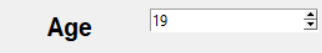
The next step involves adding a spinbox entry, which will allow users to enter a numeric value (their age) from a fixed selection of values. The spinbox entry is linked to an integer-valued variable by the textvariable option. Two further options also specify the minimum and maximum values that can be selected from. Note the use of an underscore at the from_ option – this is avoid a name class with the builtin from keyword.
age_label = Label(left_frame, text="Age", justify="center", font=("-size", 15, "-weight", "bold"))
age_label.grid(row=2, column=0, ipady=5)
age = IntVar()
age_entry = Spinbox(left_frame, textvariable=age, from_=0, to=100)
age_entry.grid(row=2, column=1, padx=5, pady=(0, 10), sticky=tkinter.E)
A screenshot of the resulting spin box is shown below.
Step 5: Adding a Combo box
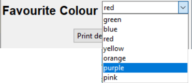
Step 5 involves adding a Combo box to the application, which allows the user to select from a predefined list of choices. In this case the Combo box provides a list of colours that the user can choose from to pick their favourite colour.
The Combobox widget is linked to the colour string variable using the textvariable option. The values option links to the list used to store the available colours.
colour_label = Label(left_frame, text="Favourite Colour", justify="right", font=("-size", 15, "-weight", "bold"))
colour_label.grid(row=3, column=0, ipady=5)
colour = StringVar()
colour_list = [
    'green',
    'blue',
    'red',
    'yellow',
    'orange',
    'purple',
    'pink'
]
colour_entry = Combobox(left_frame, textvariable=colour, values=colour_list)
colour_entry.grid(row=3, column=1, padx=5, pady=(0, 10), sticky=tkinter.E)
The screenshot below shows the combo box being used to select the user’s favourite colour. When clicked on, a menu drops down from the entry boxv allowing the user to select from the available colours.
Step 6: Date entry
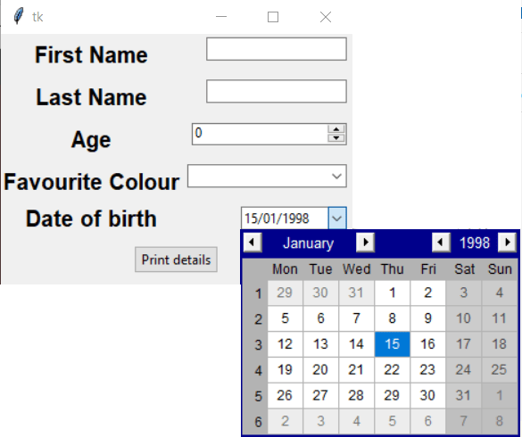
The DateEntry widget is used in this step to enter the user’s birthday. To access the DateEntry widget – together with its associated calendar widget, we need to import the tkcalendar package. This import code should be placed near the top of the file after the other import commands.
from tkcalendar import Calendar, DateEntry
The locale argument is configured so that the dates are displayed using Australian date formatting (en_AU). The year argument is used to set the year that the DateEntry will start at when it is first opened. Similar arguments are included for setting the initial day and the month. The date_pattern argument is used to specify the format that the dates will be displayed in. In this case the day and month will both be displayed using two digits, while the year will be displayed using four digits.
dob_label = Label(left_frame, text="Date of birth", justify="right", font=("-size", 15, "-weight", "bold"))
dob_label.grid(row=4, column=0)
dob_entry = DateEntry(left_frame, width=12, locale="en_AU", background='darkblue', foreground='white', borderwidth=2, year=2000, month=1, day=1, date_pattern = 'dd/mm/y')
dob_entry.grid(row=4, column=1, padx=5, sticky=tkinter.E)
The resulting date entry box is shown below.
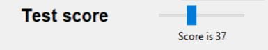
Step 7: Using a scale widget
For step 7 we use a scale widget to introduce a slider that can be used to select a test score between 0 and 100. Like the Spinbox widget, the Scale widget includes options for setting the minimum and maximum values for the slide. The variable argument links the value of the slider to an integer valued variable. The command argument links the slider to a function that is called whenever the slider is moved. A Label widget is used to display the value of the test score – this will be updated when the slider is moved.
test_score_label = Label(left_frame, text="Test score", font=("-size", 15, "-weight", "bold"))
test_score_label.grid(row=5, column=0)
testScore = IntVar()
test_score_scale = Scale(left_frame, from_=0, to=100, orient=HORIZONTAL, variable=testScore, command=update_score_display)
test_score_scale.grid(row=5, column=1)
test_score_display = Label(left_frame, text="Score is 0")
test_score_display.grid(row=6, column=1)
The function update_score_display is called whenever the slider is moved. This function updates the text displayed in the test score display label by getting the current value of the test score variable. The function, as shown below, is placed after any import commands with other function definitions.
def update_score_display(event):
    test_score_display.config(text="Score is "+ str(testScore.get()))
A screenshot of the resulting slider is shown below.
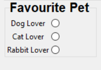
Step 8: Radio buttons
Radio buttons allow the user to make a single selection from a predefined list of choices. The selection is made by choosing the appropriate button. For our application users will select their favourite pet by clicking the appropriate button.
The radio buttons are grouped together using a LabelFrame, which as its name suggests is a frame that includes a text label.
A string-valued variable is used to store the value of the favourite pet – this variable is then linked to each of the radio buttons.
fave_animal = StringVar()
pet_frame = LabelFrame(right_frame, text="Favourite Pet")
pet_frame.grid(row=0, column=0, padx=10)
dog_lover_label= Label(pet_frame, text="Dog Lover")
dog_lover_label.grid(row=0, column=0)
dog_lover_select = Radiobutton(pet_frame, textvariable=fave_animal, value="dog")
dog_lover_select.grid(row=0, column=1)
cat_lover_label = Label(pet_frame, text="Cat Lover")
cat_lover_label.grid(row=1, column=0)
cat_lover_select = Radiobutton(pet_frame, textvariable=fave_animal, value="cat")
cat_lover_select.grid(row=1, column=1)
rabbit_lover_label = Label(pet_frame, text="Rabbit Lover")
rabbit_lover_label.grid(row=2, column=0)
rabbit_lover_select = Radiobutton(pet_frame, textvariable=fave_animal, value="rabbit")
rabbit_lover_select.grid(row=2, column=1)
The resulting label frame containing three labelled radio buttons is shown below.
Step 9: Adding check buttons
In this step check buttons are used to allow the user to select zero or more showbags. The check buttons are grouped together in a labelled frame and placed below the radio buttons frame. For each option there is an associated Boolean-valued variable that switches between true and false, with the default value in this case being false. Checkbutton widgets include a text label and a variable option which associates with the corresponding Boolean-valued variable.
showbag_frame = LabelFrame(right_frame, text="Showbag Order")
showbag_frame.grid(row=1, column=0, padx=10, pady=10)

warheads = BooleanVar()
warheads_select = Checkbutton(showbag_frame, text="Warheads", variable=warheads)
warheads_select.grid(row=0, column=0, sticky=W)

freddo = BooleanVar()
freddo_select = Checkbutton(showbag_frame, text="Freddo", variable=freddo)
freddo_select.grid(row=1, column=0, sticky=W)

blues_clues = BooleanVar()
blues_clues_select = Checkbutton(showbag_frame, text="Blue's Clues", variable=blues_clues)
blues_clues_select.grid(row=2, column=0, sticky=W)
Final application
A screenshot of the final application is shown below.
Below is a full code listing.
import tkinter as tk
from tkinter import *
from tkinter import messagebox
from tkinter.ttk import *
from tkcalendar import Calendar, DateEntry


def print_details():
    print(first_name.get(), last_name.get())
    messagebox.showinfo("Details", "hello " + str(first_name.get()) + " " + str(last_name.get()))

def update_score_display(event):
    test_score_display.config(text="Score is "+ str(testScore.get()))
# create the main application window
root = Tk()

# create a frame for a variety of entry and scale widgets
left_frame = Frame(root)
left_frame.grid(row=0, column=0)

right_frame = Frame(root)
right_frame.grid(row=0, column=1, sticky=N)

button_frame = Frame(root)
button_frame.grid(row=1, column=0, columnspan=2)
# label and entry widgets used to enter information. Values linked to string variable.
first_name_label = Label(left_frame, text="First Name", justify="center", font=("-size", 15, "-weight", "bold"))
first_name_label.grid(row=0, column=0, padx=5, pady=5)
first_name = StringVar()
first_name_entry = Entry(left_frame, textvariable=first_name)
first_name_entry.grid(row=0, column=1, padx=5, pady=(0, 10), sticky=tk.E)

last_name_label = Label(left_frame, text="Last Name", justify="center", font=("-size", 15, "-weight", "bold"))
last_name_label.grid(row=1, column=0, ipady=5)
last_name = StringVar()
last_name_entry = Entry(left_frame, textvariable=last_name)
last_name_entry.grid(row=1, column=1, padx=5, pady=(0, 10), sticky=tk.E)


print_button = Button(button_frame, text="Print details", command=print_details)
print_button.grid(row=0, column=0, padx=5, pady=10)

age_label = Label(left_frame, text="Age", justify="center", font=("-size", 15, "-weight", "bold"))
age_label.grid(row=2, column=0, ipady=5)
age = IntVar()
age_entry = Spinbox(left_frame, textvariable=age, from_=0, to=100)
age_entry.grid(row=2, column=1, padx=5, pady=(0, 10), sticky=tk.E)

colour_label = Label(left_frame, text="Favourite Colour", justify="right", font=("-size", 15, "-weight", "bold"))
colour_label.grid(row=3, column=0, ipady=5)
colour = StringVar()
colour_list = [
    'green',
    'blue',
    'red',
    'yellow',
    'orange',
    'purple',
    'pink'
]
colour_entry = Combobox(left_frame, textvariable=colour, values=colour_list)
colour_entry.grid(row=3, column=1, padx=5, pady=(0, 10), sticky=tk.E)

dob_label = Label(left_frame, text="Date of birth", justify="right", font=("-size", 15, "-weight", "bold"))
dob_label.grid(row=4, column=0)
dob_entry = DateEntry(left_frame, width=12, locale="en_AU", background='darkblue', foreground='white', borderwidth=2, year=2000)

dob_entry.grid(row=4, column=1, padx=5, sticky=tk.E)

test_score_label = Label(left_frame, text="Test score", font=("-size", 15, "-weight", "bold"))
test_score_label.grid(row=5, column=0)
testScore = IntVar()
test_score_scale = Scale(left_frame, from_=0, to=100, orient=HORIZONTAL, variable=testScore, command=update_score_display)
test_score_scale.grid(row=5, column=1)
test_score_display = Label(left_frame, text="Score is 0")
test_score_display.grid(row=6, column=1)

s = Style()
s.configure('TLabelframe.Label', font=("-size", 15, "-weight", "bold"))

fave_animal = StringVar()
pet_frame = LabelFrame(right_frame, text="Favourite Pet")
pet_frame.grid(row=0, column=0, padx=10)
dog_lover_label= Label(pet_frame, text="Dog Lover")
dog_lover_label.grid(row=0, column=0)
dog_lover_select = Radiobutton(pet_frame, textvariable=fave_animal, value="dog")
dog_lover_select.grid(row=0, column=1)
cat_lover_label = Label(pet_frame, text="Cat Lover")
cat_lover_label.grid(row=1, column=0)
cat_lover_select = Radiobutton(pet_frame, textvariable=fave_animal, value="cat")
cat_lover_select.grid(row=1, column=1)
rabbit_lover_label = Label(pet_frame, text="Rabbit Lover")
rabbit_lover_label.grid(row=2, column=0)
rabbit_lover_select = Radiobutton(pet_frame, textvariable=fave_animal, value="rabbit")
rabbit_lover_select.grid(row=2, column=1)

showbag_frame = LabelFrame(right_frame, text="Showbag Order")
showbag_frame.grid(row=1, column=0, padx=10, pady=10)

warheads = BooleanVar()
warheads_select = Checkbutton(showbag_frame, text="Warheads", variable=warheads)
warheads_select.grid(row=0, column=0, sticky=W)

freddo = BooleanVar()
freddo_select = Checkbutton(showbag_frame, text="Freddo", variable=freddo)
freddo_select.grid(row=1, column=0, sticky=W)

blues_clues = BooleanVar()
blues_clues_select = Checkbutton(showbag_frame, text="Blue's Clues", variable=blues_clues)
blues_clues_select.grid(row=2, column=0, sticky=W)

root.mainloop()
.jpg)


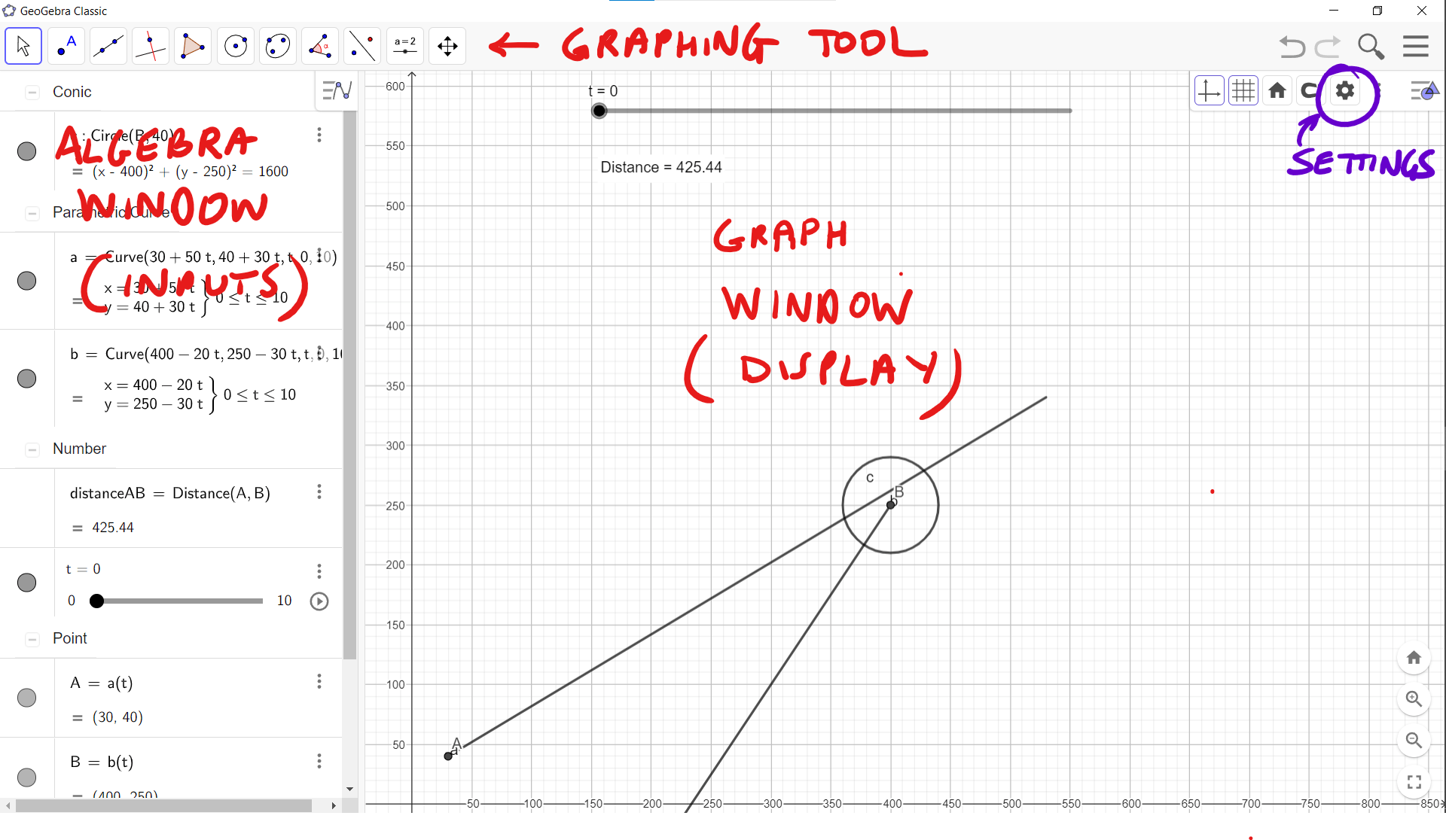
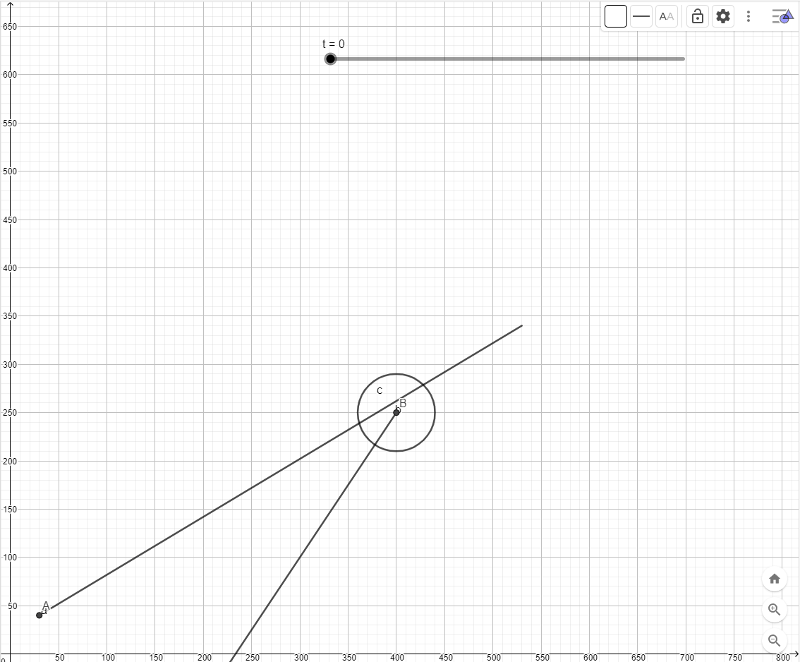
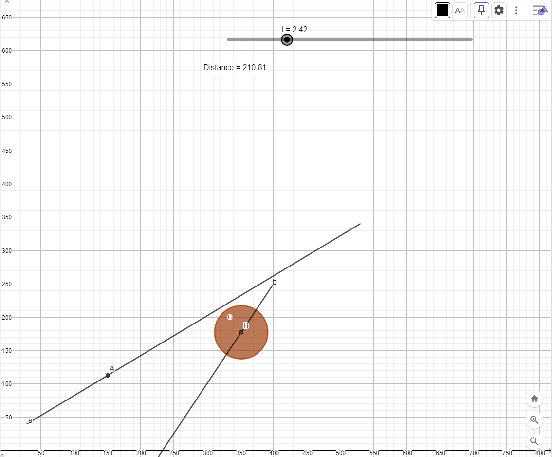
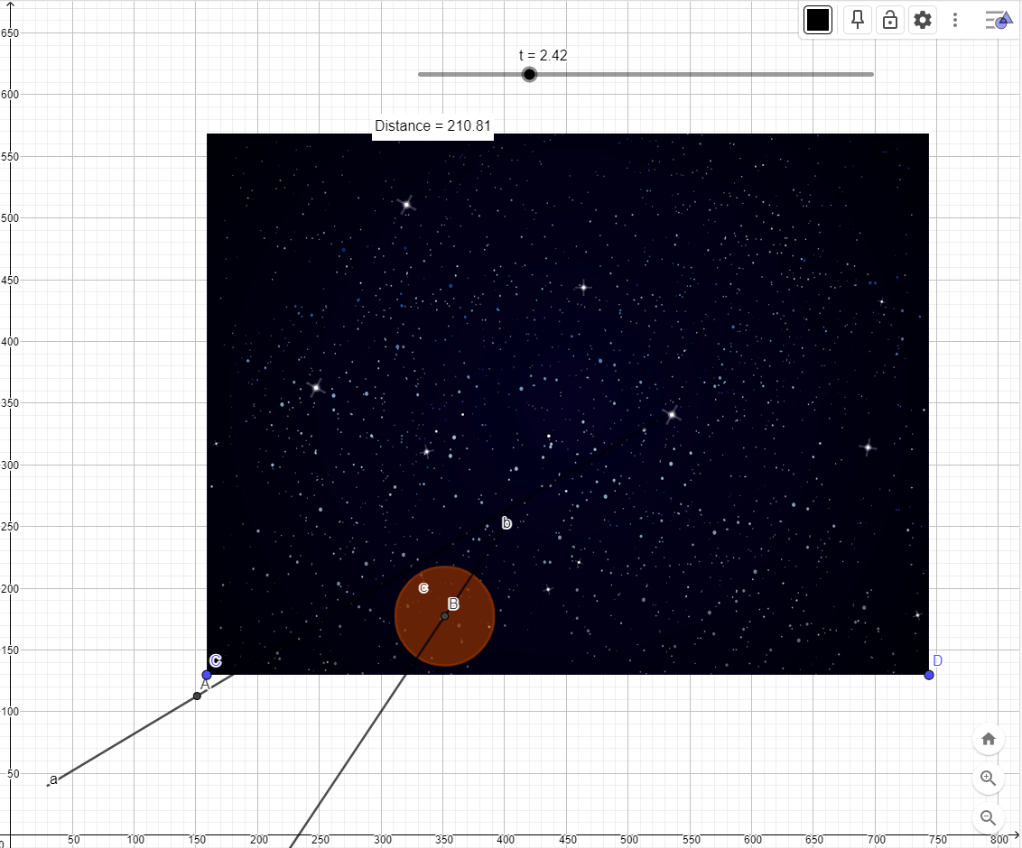
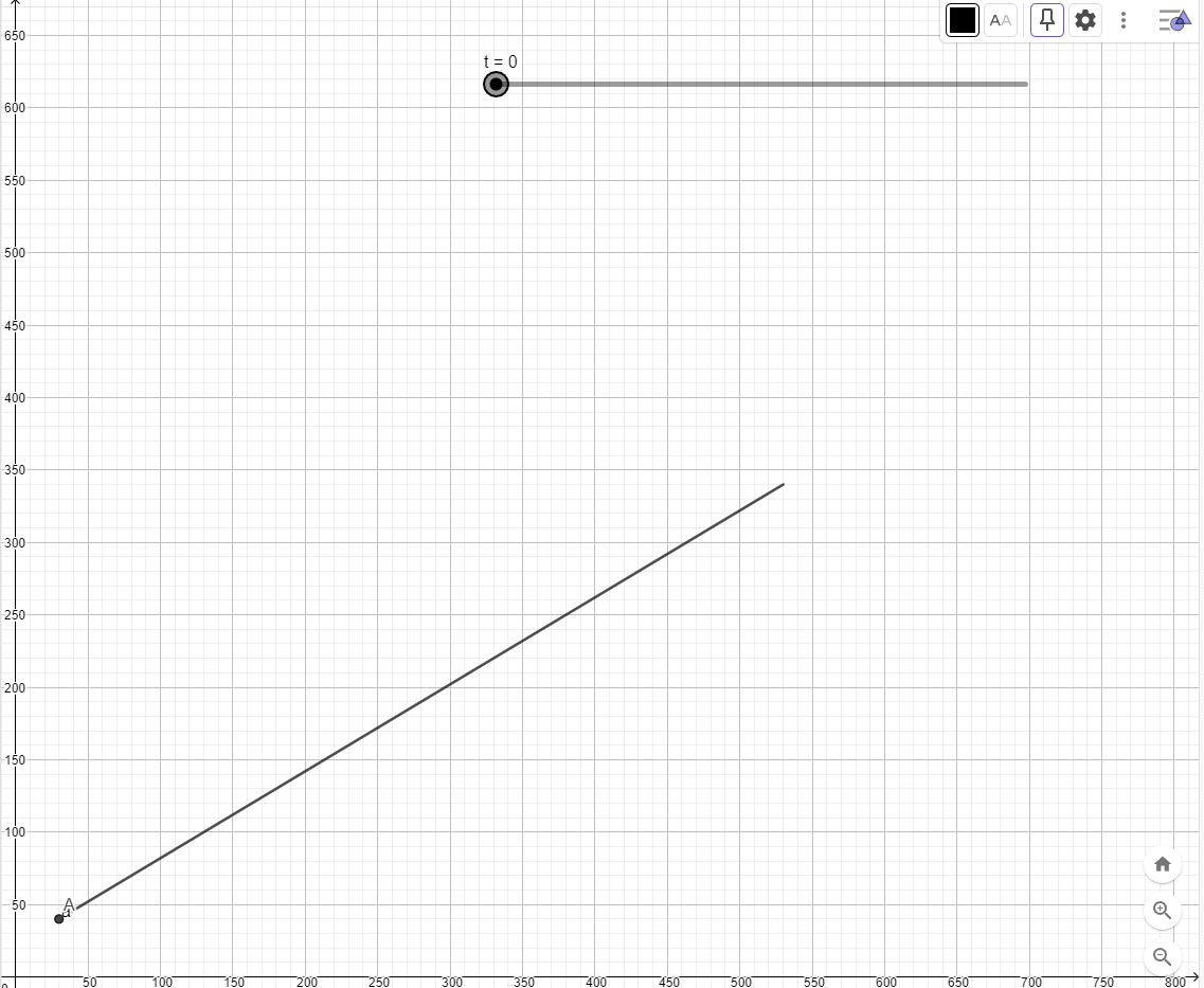
![\vec{r_A} = [30, 40]+t[50,30]](https://s0.wp.com/latex.php?latex=%5Cvec%7Br_A%7D+%3D+%5B30%2C+40%5D%2Bt%5B50%2C30%5D&bg=ffffff&fg=000000&s=0 "\vec{r_A} = [30, 40]+t[50,30]")
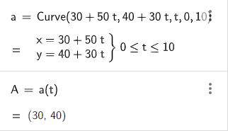
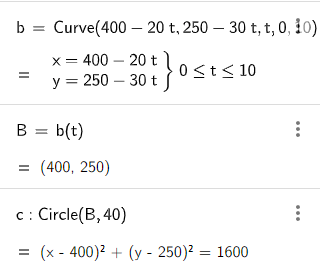
![\vec{r_A} = [400, 250]+t[-20,-30]](https://s0.wp.com/latex.php?latex=%5Cvec%7Br_A%7D+%3D+%5B400%2C+250%5D%2Bt%5B-20%2C-30%5D&bg=ffffff&fg=000000&s=0 "\vec{r_A} = [400, 250]+t[-20,-30]")